wavepy.utils

Utility functions to help.

Functions:

crop_matrix_at_indexes(input_matrix, ...)	Alias for np.copy(inputMatrix[i_min:i_max, j_min:j_max])
date_now_str()	Returns the current date as a string in the format YYmmDD.
datetime_now_str()	Returns the current date and time as a string in the format YYmmDD_HHMMSS.
dummy_images([imagetype, shape])	Dummy images for simple tests.
find_nearest_value(input_array, value)	Alias for
find_nearest_value_index(input_array, value)	Similar to wavepy.utils.find_nearest_value(), but returns
fouriercoordmatrix(npointsx, deltax, ...)	For back compability
fouriercoordvec(npoints, delta)	For back compability
graphical_roi_idx(zmatrix[, verbose, ...])	Function to define a rectangular region of interest (ROI) in an image.
graphical_select_point_idx(zmatrix[, ...])	Plot a 2D array and allow to pick a point in the image.
h5_list_of_groups(h5file)	Get the names of all groups and subgroups in a hdf5 file.
load_ini_file(inifname)	Parameters:inifname (str) – name of the *.ini file.
nan_mask_threshold(input_matrix[, threshold])	Calculate a square mask for array above OR below a threshold
plot_profile(xmatrix, ymatrix, zmatrix[, ...])	Plot contourf in the main graph plus profiles over vertical and horizontal lines defined with mouse.
print_blue(message)	Print with colored characters.
print_color(message[, color, highlights, attrs])	Print with colored characters.
print_red(message)	Print with colored characters.
progress_bar4pmap(res[, sleep_time])	Progress bar from tqdm to be used with the function multiprocessing.starmap_async().
realcoordmatrix(npointsx, deltax, npointsy, ...)	Build a matrix (2D array) with real space coordinates based on the number of points and bin (pixels) size.
realcoordmatrix_fromvec(xvec, yvec)	Alias for np.meshgrid(xvec, yvec)
realcoordvec(npoints, delta)	Build a vector with real space coordinates based on the number of points and bin (pixels) size.
rotate_img_graphical(array2D[, order, mode, ...])	GUI to rotate an image
select_dir([message_to_print, pattern])	List subdirectories of the current working directory, and expected the user to choose one of them.
select_file([pattern, message_to_print])	List files under the subdirectories of the current working directory, and expected the user to choose one of them.
time_now_str()	Returns the current time as a string in the format HHMMSS.

wavepy.utils.print_color(message, color='red', highlights='on_white', attrs='')

Print with colored characters. It is only a alias for colored print using the package termcolor and equals to:

print(termcolor.colored(message, color, highlights, attrs=attrs))

See options at https://pypi.python.org/pypi/termcolor

Parameters:

• message (str) – Message to print.
• color, highlights (str)
• attrs (list)

wavepy.utils.print_red(message)

Print with colored characters. It is only a alias for colored print using the package termcolor and equals to:

print(termcolor.colored(message, color='red'))

Parameters:message (str) – Message to print.

wavepy.utils.print_blue(message)

Print with colored characters. It is only a alias for colored print using the package termcolor and equals to:

print(termcolor.colored(message, color='blue'))

Parameters:message (str) – Message to print.

wavepy.utils.plot_profile(xmatrix, ymatrix, zmatrix, xlabel='x', ylabel='y', zlabel='z', title='Title', xo=None, yo=None, xunit='', yunit='', do_fwhm=True, arg4main=None, arg4top=None, arg4side=None)

Plot contourf in the main graph plus profiles over vertical and horizontal lines defined with mouse.

Parameters:

• xmatrix, ymatrix (ndarray) – x and y matrix coordinates generated with numpy.meshgrid()
• zmatrix (ndarray) – Matrix with the data. Note that xmatrix, ymatrix and zmatrix must have the same shape
• xlabel, ylabel, zlabel (str, optional) – Labels for the axes x, y and z.
• title (str, optional) – title for the main graph #BUG: sometimes this title disappear
• xo, yo (float, optional) – if equal to None, it allows to use the mouse to choose the vertical and horizontal lines for the profile. If not None, the profiles lines are are centered at (xo,yo)
• xunit, yunit (str, optional) – String to be shown after the values in the small text box
• do_fwhm (Boolean, optional) – Calculate and print the FWHM in the figure. The script to calculate the FWHM is not very robust, it works well if only one well defined peak is present. Turn this off by setting this var to False
• *arg4main – *args for the main graph
• *arg4top – *args for the top graph
• *arg4side – *args for the side graph

Returns:

• ax_main, ax_top, ax_side (matplotlib.axes) – return the axes in case one wants to modify them.
• delta_x, delta_y (float)

Example

>>> import numpy as np
>>> import wavepy.utils as wpu
>>> xx, yy = np.meshgrid(np.linspace(-1, 1, 101), np.linspace(-1, 1, 101))
>>> wpu.plot_profile(xx, yy, np.exp(-(xx**2+yy**2)/.2))

Animation of the example above:

wavepy.utils.select_file(pattern='*', message_to_print=None)

List files under the subdirectories of the current working directory, and expected the user to choose one of them.

The list of files is of the form number: filename. The user choose the file by typing the number of the desired filename.

Parameters:

• pattern (str) – list only files with this patter. Similar to pattern in the linux comands ls, grep, etc
• message_to_print (str, optional)

Returns:

filename (str) – path and name of the file

Example

>>>  select_file('*.dat')

wavepy.utils.select_dir(message_to_print=None, pattern='**/')

List subdirectories of the current working directory, and expected the user to choose one of them.

The list of files is of the form number: filename. The user choose the file by typing the number of the desired filename.

Similar to wavepy.utils.select_file()

Parameters:message_to_print (str, optional) Returns:str – directory path

See also

wavepy.utils.select_file()

wavepy.utils.nan_mask_threshold(input_matrix, threshold=0.0)

Calculate a square mask for array above OR below a threshold

Parameters:

• input_matrix (ndarray) – 2 dimensional (or n-dimensional?) numpy.array to be masked
• threshold (float) – threshold for masking. If real (imaginary) value, values below(above) the threshold are set to NAN

Returns:

ndarray – array with values either equal to 1 or NAN.

Example

To use as a mask for array use:

>>> mask = nan_mask_threshold(input_array, threshold)
>>> masked_array = input_array*mask

Notes

• Note that array[mask] will return only the values where mask == 1.
• Also note that this is NOT the same as the masked arrays in numpy.

wavepy.utils.crop_matrix_at_indexes(input_matrix, list_of_indexes)

Alias for np.copy(inputMatrix[i_min:i_max, j_min:j_max])

Parameters:

• input_matrix (ndarray) – 2 dimensional array
• list_of_indexes (list) – list in the format [i_min, i_max, j_min, j_max]

Returns:

ndarray – copy of the sub-region inputMatrix[i_min:i_max, j_min:j_max] of the inputMatrix.

Warning

Note the difference of copy and view in Numpy.

wavepy.utils.crop_graphic(xvec=None, yvec=None, zmatrix=None, verbose=False, kargs4graph={})

Function to crop an image to the ROI selected using the mouse.

wavepy.utils.graphical_roi_idx() is first used to plot and select the ROI. The function then returns the croped version of the matrix, the cropped coordinate vectors x and y, and the indexes [i_min, i_max, j_min,_j_max]

Parameters:

• xvec, yvec (1D ndarray) – vector with the coordinates x and y. See below how the returned variables change dependnding whether these vectors are provided.
• zmatrix (2D numpy array) – image to be croped, as an 2D ndarray
• **kargs4graph – kargs for main graph

Returns:

• 1D ndarray, 1D ndarray – cropped coordinate vectors x and y. These two vectors are only returned the input vectors xvec and xvec are provided
• 2D ndarray – cropped image
• list – indexes of the crop [i_min, i_max, j_min,_j_max]. Useful when the same crop must be applies to other images

Examples

>>> import numpy as np
>>> import matplotlib as plt
>>> xVec = np.arange(0.,101)
>>> yVec = np.arange(0.,101)
>>> img = dummy_images('Shapes', size=(101,101), FWHM_x = .5, FWHM_y=1.0)
>>> (imgCroped, idx4crop) = crop_graphic(zmatrix=img)
>>> plt.imshow(imgCroped, cmap='Spectral')
>>> (xVecCroped,
>>>  yVecCroped,
>>>  imgCroped, idx4crop) = crop_graphic(xVec, yVec, img)
>>> plt.imshow(imgCroped, cmap='Spectral',
>>>            extent=np.array([xVecCroped[0], xVecCroped[-1],
>>>                             yVecCroped[0], yVecCroped[-1]])

See also

wavepy.utils.crop_graphic_image() wavepy.utils.graphical_roi_idx()

wavepy.utils.crop_graphic_image(image, verbose=False, **kargs4graph)

Similar to wavepy.utils.crop_graphic(), but only for the main matrix (and not for the x and y vectors). The function then returns the croped version of the image and the indexes [i_min, i_max, j_min,_j_max]

Parameters:

• zmatrix (2D numpy array) – image to be croped, as an 2D ndarray
• **kargs4graph – kargs for main graph

Returns:

• 2D ndarray – cropped image
• list – indexes of the crop [i_min, i_max, j_min,_j_max]. Useful when the same crop must be applies to other images

See also

wavepy.utils.crop_graphic() wavepy.utils.graphical_roi_idx()

wavepy.utils.crop_graphic_image(image, verbose=False, **kargs4graph)

Similar to wavepy.utils.crop_graphic(), but only for the main matrix (and not for the x and y vectors). The function then returns the croped version of the image and the indexes [i_min, i_max, j_min,_j_max]

Parameters:

• zmatrix (2D numpy array) – image to be croped, as an 2D ndarray
• **kargs4graph – kargs for main graph

Returns:

• 2D ndarray – cropped image
• list – indexes of the crop [i_min, i_max, j_min,_j_max]. Useful when the same crop must be applies to other images

See also

wavepy.utils.crop_graphic() wavepy.utils.graphical_roi_idx()

wavepy.utils.graphical_select_point_idx(zmatrix, verbose=False, kargs4graph={})

Plot a 2D array and allow to pick a point in the image. Returns the last selected position x and y of the choosen point

Parameters:

• zmatrix (2D numpy array) – main image
• verbose (Boolean) – verbose mode
• **kargs4graph – kargs for main graph

Returns:

int, int – two integers with the point indexes x and y

Example

>>> jo, io = graphical_select_point_idx(array2D)
>>> value = array2D[io, jo]

See also

wavepy.utils.graphical_roi_idx()

wavepy.utils.find_nearest_value(input_array, value)

Alias for input_array.flatten()[np.argmin(np.abs(input_array.flatten() - value))]

In a array of float numbers, due to the precision, it is impossible to find exact values. For instance something like array1[array2==0.0] might fail because the zero values in the float array array2 are actually something like 0.0004324235 (fictious value).

This function will return the value in the array that is the nearest to the parameter value.

Parameters:

• input_array (ndarray)
• value (float)

Returns:

ndarray

Example

>>> foo = dummy_images('NormalDist')
>>> find_nearest_value(foo, 0.5000)
0.50003537554879007

See also

wavepy:utils:find_nearest_value_index()

wavepy.utils.find_nearest_value_index(input_array, value)

Similar to wavepy.utils.find_nearest_value(), but returns the index of the nearest value (instead of the value itself)

Parameters:

• input_array (ndarray)
• value (float)

Returns:

tuple of ndarray – each array have the index of the nearest value in each dimension

Note

In principle it has no limit of the number of dimensions.

Example

>>> foo = dummy_images('NormalDist')
>>> find_nearest_value(foo, 0.5000)
0.50003537554879007
>>> (i_index, j_index) = find_nearest_value_index(foo, 0.500)
>>> foo[i_index[:], j_index[:]]
array([ 0.50003538,  0.50003538,  0.50003538,  0.50003538])

See also

wavepy:utils:find_nearest_value()

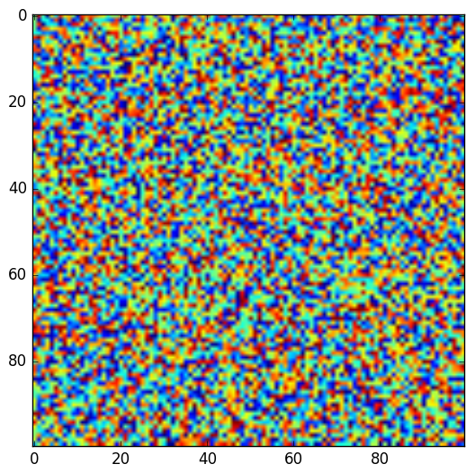
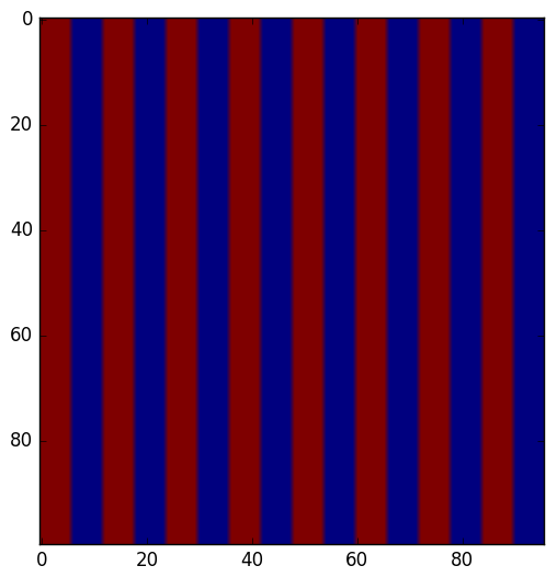
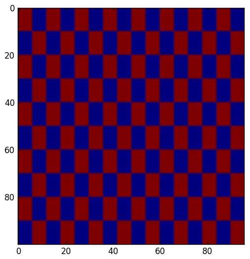
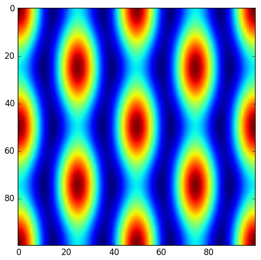
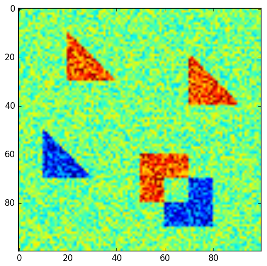
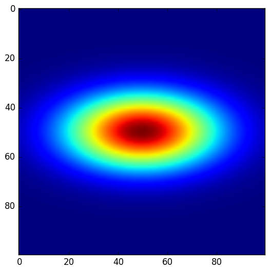
wavepy.utils.dummy_images(imagetype=None, shape=(100, 100), **kwargs)

Dummy images for simple tests.

Parameters:

• imagetype (str) – See options Below
• shape (tuple) – Shape of the image. Similar to numpy.shape
• kwargs – keyword arguments depending on the image type.

Image types

• Noise (default): alias for np.random.random(shape)

• Stripes: kwargs: nLinesH, nLinesV

• SumOfHarmonics: image is defined by: .. math:: sum_{ij} Amp_{ij} cos (2 pi i y) cos (2 pi j x).

  • Note that x and y are assumed to in the range [-1, 1]. The keyword kwargs: harmAmpl is a 2D list that can be used to set the values for Amp_ij, see Examples.

• Shapes: see Examples. kwargs=noise, amplitude of noise to be added to the image

• NormalDist: Normal distribution where it is assumed that x and y are in the interval [-1,1]. keywords: FWHM_x, FWHM_y

Returns:2D ndarray

Examples

>>> import matplotlib.pyplot as plt
>>> plt.imshow(dummy_images())

is the same than

>>> plt.imshow(dummy_images('Noise'))

>>> plt.imshow(dummy_images('Stripes', nLinesV=5))

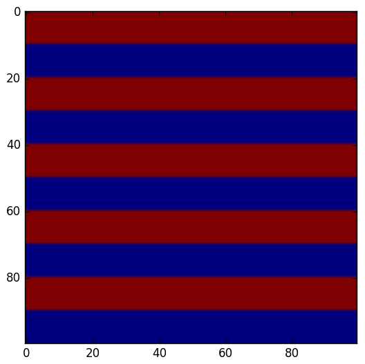
>>> plt.imshow(dummy_images('Stripes', nLinesH=8))

>>> plt.imshow(dummy_images('Checked', nLinesH=8, nLinesV=5))

>>> plt.imshow(dummy_images('SumOfHarmonics', harmAmpl=[[1,0,1],[0,1,0]]))

>>> plt.imshow(dummy_images('Shapes', noise = 1))

>>> plt.imshow(dummy_images('NormalDist', FWHM_x = .5, FWHM_y=1.0))

wavepy.utils.graphical_roi_idx(zmatrix, verbose=False, kargs4graph={})

Function to define a rectangular region of interest (ROI) in an image.

The image is plotted and, using the mouse, the user select the region of interest (ROI). The ROI is ploted as an transparent rectangular region. When the image is closed the function returns the indexes [i_min, i_max, j_min, j_max] of the ROI.

Parameters:

• input_array (ndarray)
• verbose (Boolean) – In the verbose mode it is printed some additional infomations, like the ROI indexes, as the user select different ROI’s
• **kargs4graph – Options for the main graph. WARNING: not tested very well

Returns:

list – indexes of the ROI [i_min, i_max, j_min,_j_max]. Useful when the same crop must be applies to other images

Note

In principle it has no limit of the number of dimensions.

Example

See example at wavepy:utils:crop_graphic()

See also

wavepy:utils:crop_graphic()

wavepy.utils.crop_graphic(xvec=None, yvec=None, zmatrix=None, verbose=False, kargs4graph={})

Function to crop an image to the ROI selected using the mouse.

wavepy.utils.graphical_roi_idx() is first used to plot and select the ROI. The function then returns the croped version of the matrix, the cropped coordinate vectors x and y, and the indexes [i_min, i_max, j_min,_j_max]

Parameters:

• xvec, yvec (1D ndarray) – vector with the coordinates x and y. See below how the returned variables change dependnding whether these vectors are provided.
• zmatrix (2D numpy array) – image to be croped, as an 2D ndarray
• **kargs4graph – kargs for main graph

Returns:

• 1D ndarray, 1D ndarray – cropped coordinate vectors x and y. These two vectors are only returned the input vectors xvec and xvec are provided
• 2D ndarray – cropped image
• list – indexes of the crop [i_min, i_max, j_min,_j_max]. Useful when the same crop must be applies to other images

Examples

>>> import numpy as np
>>> import matplotlib as plt
>>> xVec = np.arange(0.,101)
>>> yVec = np.arange(0.,101)
>>> img = dummy_images('Shapes', size=(101,101), FWHM_x = .5, FWHM_y=1.0)
>>> (imgCroped, idx4crop) = crop_graphic(zmatrix=img)
>>> plt.imshow(imgCroped, cmap='Spectral')
>>> (xVecCroped,
>>>  yVecCroped,
>>>  imgCroped, idx4crop) = crop_graphic(xVec, yVec, img)
>>> plt.imshow(imgCroped, cmap='Spectral',
>>>            extent=np.array([xVecCroped[0], xVecCroped[-1],
>>>                             yVecCroped[0], yVecCroped[-1]])

See also

wavepy.utils.crop_graphic_image() wavepy.utils.graphical_roi_idx()

wavepy.utils.choose_unit(array)

Script to choose good(best) units in engineering notation for a ndarray.

For a given input array, the function returns factor and unit according to

\[10^{n} < \max(array) < 10^{n + 3}\]

n	factor (float)	unit(str)
0	1.0	'' empty string
-9	10^-9	n
-6	10^-6	r'\mu'
-3	10^-3	m
+3	10^-6	k
+6	10^-9	M
+9	10^-6	G

n=-6 returns \mu since this is the latex syntax for micro. See Example.

Parameters:array (ndarray) – array from where to choose proper unit. Returns:float, unit – Multiplication Factor and strig for unit

Example

>>> array1 = np.linspace(0,100e-6,101)
>>> array2 = array1*1e10
>>> factor1, unit1 = choose_unit(array1)
>>> factor2, unit2 = choose_unit(array2)
>>> plt.plot(array1*factor1,array2*factor2)
>>> plt.xlabel(r'${0} m$'.format(unit1))
>>> plt.ylabel(r'${0} m$'.format(unit2))

The syntax r'$ string $ ' is necessary to use latex commands in the matplotlib labels.

wavepy.utils.datetime_now_str()

Returns the current date and time as a string in the format YYmmDD_HHMMSS. Alias for time.strftime("%Y%m%d_%H%M%S").

Returns:str

wavepy.utils.time_now_str()

Returns the current time as a string in the format HHMMSS. Alias for time.strftime("%H%M%S").

Returns:str

wavepy.utils.date_now_str()

Returns the current date as a string in the format YYmmDD. Alias for time.strftime("%Y%m%d").

Returns:str

wavepy.utils.realcoordvec(npoints, delta)

Build a vector with real space coordinates based on the number of points and bin (pixels) size.

Alias for np.mgrid[-npoints/2*delta:npoints/2*delta-delta:npoints*1j]

Parameters:

• npoints (int) – number of points
• delta (float) – vector with the values of x

Returns:

ndarray – vector (1D array) with real coordinates

Example

>>> realcoordvec(10,1)
array([-5., -4., -3., -2., -1.,  0.,  1.,  2.,  3.,  4.])

See also

wavepy.utils.realcoordmatrix_fromvec() wavepy.utils.realcoordmatrix()

wavepy.utils.realcoordmatrix_fromvec(xvec, yvec)

Alias for np.meshgrid(xvec, yvec)

Parameters:xvec, yvec (ndarray) – vector (1D array) with real coordinates Returns:ndarray – 2 matrices (1D array) with real coordinates

Example

>>> vecx = realcoordvec(3,1)
>>> vecy = realcoordvec(4,1)
>>> realcoordmatrix_fromvec(vecx, vecy)
[array([[-1.5, -0.5,  0.5],
[-1.5, -0.5,  0.5],
[-1.5, -0.5,  0.5],
[-1.5, -0.5,  0.5]]),
array([[-2., -2., -2.],
[-1., -1., -1.],
[ 0.,  0.,  0.],
[ 1.,  1.,  1.]])]

See also

wavepy.utils.realcoordvec() wavepy.utils.realcoordmatrix()

wavepy.utils.realcoordmatrix(npointsx, deltax, npointsy, deltay)

Build a matrix (2D array) with real space coordinates based on the number of points and bin (pixels) size.

Alias for realcoordmatrix_fromvec(realcoordvec(nx, delx), realcoordvec(ny, dely))

Parameters:

• npointsx, npointsy (int) – number of points in the x and y directions
• deltax, deltay (float) – step size in the x and y directions

Returns:

ndarray, ndarray – 2 matrices (2D array) with real coordinates

Example

>>> realcoordmatrix(3,1,4,1)
[array([[-1.5, -0.5,  0.5], [-1.5, -0.5,  0.5], [-1.5, -0.5,  0.5],
[-1.5, -0.5,  0.5]]), array([[-2., -2., -2.], [-1., -1., -1.],
[ 0.,  0.,  0.], [ 1.,  1.,  1.]])]

See also

wavepy.utils.realcoordvec() wavepy.utils.realcoordmatrix_fromvec()

wavepy.utils.reciprocalcoordvec(npoints, delta)

Create coordinates in the (spatial) frequency domain based on the number of points n and the step (binning) \Delta x in the REAL SPACE. It returns a vector of frequencies with values in the interval

\[\left[ \frac{-1}{2 \Delta x} : \frac{1}{2 \Delta x} - \frac{1}{n \Delta x} \right],\]

with the same number of points.

Parameters:

• npoints (int) – number of points
• delta (float) – step size in the REAL SPACE

Returns:

ndarray

Example

>>> reciprocalcoordvec(10,1e-3)
array([-500., -400., -300., -200., -100., 0., 100., 200., 300., 400.])

See also

wavepy.utils.realcoordvec() wavepy.utils.reciprocalcoordmatrix()

wavepy.utils.reciprocalcoordmatrix(npointsx, deltax, npointsy, deltay)

Similar to wavepy.utils.reciprocalcoordvec(), but for matrices (2D arrays).

Parameters:

• npointsx, npointsy (int) – number of points in the x and y directions
• deltax, deltay (float) – step size in the x and y directions

Returns:

ndarray, ndarray – 2 matrices (2D array) with coordinates in the frequencies domain

Example

>>> reciprocalcoordmatrix(5, 1e-3, 4, 1e-3)
[array([[-500., -300., -100.,  100.,  300.],
[-500., -300., -100.,  100.,  300.],
[-500., -300., -100.,  100.,  300.],
[-500., -300., -100.,  100.,  300.]]),
array([[-500., -500., -500., -500., -500.],
[-250., -250., -250., -250., -250.],
[   0.,    0.,    0.,    0.,    0.],
[ 250.,  250.,  250.,  250.,  250.]])]

See also

wavepy.utils.realcoordmatrix() wavepy.utils.reciprocalcoordvec()

wavepy.utils.h5_list_of_groups(h5file)

Get the names of all groups and subgroups in a hdf5 file.

Parameters:h5file (h5py file) Returns:list – list of strings with group names

Example

>>> fh5 = h5py.File(filename,'r')
>>> listOfGoups = h5_list_of_groups(fh5)
>>> for group in listOfGoups: print(group)

wavepy.utils.progress_bar4pmap(res, sleep_time=1.0)

Progress bar from tqdm to be used with the function multiprocessing.starmap_async().

It holds the program in a loop waiting multiprocessing.starmap_async() to finish

Parameters:

• res (result object of the multiprocessing.Pool class)
• sleep_time

Example

>>> from multiprocessing import Pool
>>> p = Pool()
>>> res = p.starmap_async(...)  # use your function inside brackets
>>> p.close()  # No more work
>>> progress_bar4pmap(res)

wavepy.utils.load_ini_file(inifname)

Parameters:inifname (str) – name of the *.ini file. Returns:configparser objects

Example

Example of ini file:

[Files]
image_filename = file1.tif
ref_filename = file2.tif

[Parameters]
par1 = 10.5e-5
par2 = 10, 100, 500, 600
par can have long name = 25
par3 = the value can be anything

If we create a file named .temp.ini with the example above, we can load it as:

>>> config = load_ini_file('.temp.ini')
>>> print(config['Parameters']['Par1'] )

See also

wavepy.utils.load_ini_file_terminal_dialog(), wavepy.utils.get_from_ini_file(), wavepy.utils.set_at_ini_file().

wavepy.utils.rocking_3d_figure(ax, outfname='out.ogv', elevAmp=50, azimAmpl=90, elevOffset=0, azimOffset=0, dpi=50, npoints=200, del_tmp_imgs=True)

Saves an image at different view angles and join the images to make a short animation. The movement is defined by setting the elevation and azimut angles following a sine function. The frequency of the vertical movement (elevation) is twice of the horizontal (azimute), forming a figure eight movement.

Parameters:

• ax (3D axis object) – See example below how to create this object. If None, this will use the temporary images from a previous run
• outfname (str) – output file name. Note that the extension defines the file format. This function has been tested for the formats .gif (not recomended, big files and poor quality), .mp4, .mkv and .ogv. For LibreOffice, .ogv is the recomend format.
• elevAmp (float) – amplitude of elevation movement, in degrees
• azimAmpl (float) – amplitude of azimutal movement, in degrees. If negative, the image will continually rotate around the azimute direction (no azimute rocking)
• elevOffset (float) – offset of elevation movement, in degrees
• azimOffset (float) – offset of azimutal movement, in degrees
• dpi (float) – resolution of the individual images
• npoints (int) – number of intermediary images to form the animation. More images will make the the movement slower and the animation longer.
• remove_images (float) – the program creates npoints temporary images, and this flag defines if these images are deleted or not

Example

>>> fig = plt.figure()
>>> ax = fig.add_subplot(111, projection='3d')
>>> xx = np.random.rand(npoints)*2-1
>>> yy = np.random.rand(npoints)*2-1
>>> zz = np.sinc(-(xx**2/.5**2+yy**2/1**2))
>>> ax.plot_trisurf(xx, yy, zz, cmap='viridis', linewidth=0.2, alpha = 0.8)
>>> plt.show()
>>> plt.pause(.5)
>>> # this pause is necessary to plot the first image in the main screen
>>> rocking_3d_figure(ax, 'out_080.ogv',
                      elevAmp=45, azimAmpl=45,
                      elevOffset=0, azimOffset=45, dpi=80)
>>> # example of use of the del_tmp_imgs flag
>>> rocking_3d_figure(ax, 'out_050.ogv',
                      elevAmp=60, azimAmpl=60,
                      elevOffset=10, azimOffset=45,
                      dpi=50, del_tmp_imgs=False)
>>> rocking_3d_figure(None, 'out2_050.gif',
                      del_tmp_imgs=True)